
Exercise Week 2: MD
Molecular dynamics of liquid H2O and calculations with MD integrators
The exercise of the second week contains two parts. In the first part, we will run three different classical MD simulations for liquid H2O, using:
-
The parameters reported by Praprotnik et al.
-
The fitted force field parameters we constructed in the last exercise after performing force matching
-
And finally, the fitted force field parameters at a higher temperature, i.e. at 400K
After this, we will compute radial distribution functions (RDFs) from all three MD trajectories.
The last part will be to compute the orbit of the Earth around the Sun using a Jupyter Notebook.
The required iput files can be obtained from here.
Some information regarding the input files
-
The directory
2.1-NH2O-MDcontains the input filemd.infor the classical MD simulation. -
The directory
2.2-NH2O-GOFRcontains the filegoo_exp.ALSwhich has the experimental RDF data andmultiplot_comp.agrwhich has the RDF data computed with another force field. -
The directory
2.3-MD_integratorscontains the fileexercise_lecture3_MD.ipynbwhich you can open with Jupyter Notebook.
2.1. Classical MD simulation for liquid H2O
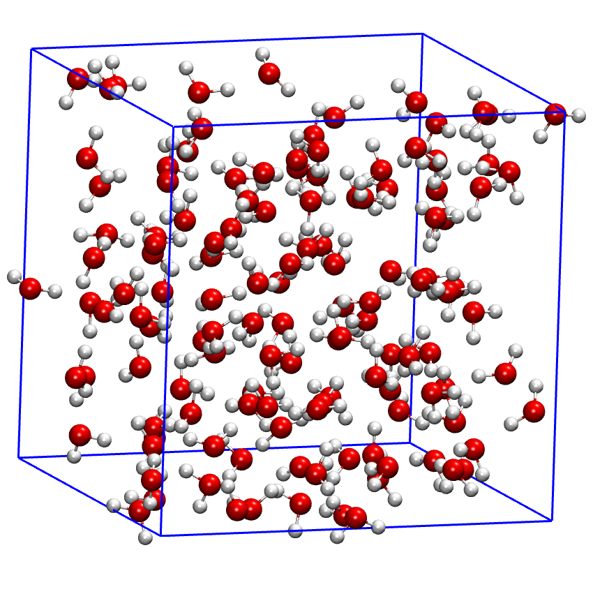
The directory 2.1-NH2O-MD contains the input file md.in. The force field parameters given by Praprotnik et al. are already used here. Copy the directory again and now replace the bond lengths, angles and charges with the fitted parameters we calculated from the last exercise after performing force matching. Start running these simulations one by one.
|
Each of the simulations will take approximately 15 minutes. You can work on your other tasks in the meantime. 🙂 |
We ran these two simulations at 300K. In order to see the effects of temperature, repeat the MD simulation with the fitted parameters using an inital temperature of 400K.
|
2.2. Calculation of radial distribution functions
Next, analyze the trajectories (run-NH2O-MD-T300.xyz) in order to calculate the radial distribution function (rdf, g(r)) as a function of temperature. Do this for all of the three MD trajectories you obtained.
VMD comes with an extension for exactly this purpose: In the VMD Main window, open Extensions → Analysis and then click on Radial Pair Distribution function g(r). In the appearing window, first select the molecule and then use Utilities → Set unit cell dimensions to let VMD know the simulation box you used. After that use Selection 1 and 2 to define the atomic types that you want to calculate the rdf for, for example element O. In order to be able to compare with the experimental data, set delta r (bin width) to 0.01.
|
After plotting the RDF, you can save the plot by clicking |
|
In the future, we will also compute IR spectrum from these MD simulations!
2.3. Calculating the orbit of the Earth around the Sun using the Verlet method
Our final exercise for the MD topic will be to calculate the orbit of the Earth around the Sun using the Verlet method. This is a programming exercise, hence you will use Jupyter Notebook.
Go to the directory 2.3-MD_integrators and open the file exercise_lecture3_MD.ipynb with Jupyter Notebook. For further information, please follow the instructions there.
References
For more MD exercises with CP2K, please look at here.